알고리즘 분류
비지도학습
- 군집화(K-means, SOM, 계층군집)
- 차원축소(주성분분석, 선형판별분석)
- 연관분석
- 자율학습 인공신경망
지도학습
- 회귀
- 로지스틱회귀
- 나이브 베이즈
- KNN
- 의사결정나무(Disicion Tree)
- 인공신경망
- 서포트벡터머신(SVM)
- 랜덤포레스트 https://ratsgo.github.io/machine%20learning/2017/03/26/tree/
✅ 실습
3주차 부터는 본격적으로 코딩을 실습을 해보고 각 알고리즘의 특성을 이해하려고 실습 위주의 학습을 진행, 구글 Colabs에서 실습을 하면서 알고리즘 옵션과 주석을 넣어 놓은 내용을 보면서 반복적으로 코딩 연습
- 각 알고리즘의 옵션에 대해 이론적으로 익히고 옵션 변경에 따라 달라지는 결과 값을 해석하는 방법을 이해하도록 했다.

✅ KNN (k-Nearest Neighborhood) : 최근접 이웃 알고리즘
하이퍼 파라미터 K값 근처 이웃의 숫자
- k-최근접 이웃 분류
- 가장 가깝게 위치하는 멤버 분류
from sklearn import neighbors, datasets
import numpy as np
import matplotlib.pyplot as plt
from matplotlib.colors import ListedColormap

iris = datasets.load_iris()

X = iris.data[:, :2]
y = iris.target

list(iris.target_names)
💡n_neighbors로 k를 지정
- x 데이터를 분류를 할 때 k개의 이웃 중 거리가 가까운 이웃의 영향을 더 많이 받도록 가중치를 설정은 weights = "distance"를 지정
- KNN의 가장 단순한 형태로 주변 5개 이웃 기준으로 범주를 예측
# k = 5 (n_neighbors)로 지정
clf = neighbors.KNeighborsClassifier(5)
clf.fit(X,y)

y_pred=clf.predict(X)

from sklearn.metrics import confusion_matrix
['setosa', 'versicolor', 'virginica']
💡confusion_matrix를 사용한 모델 예측 (정확도) 측정
- 0번 범주 1개 오답
- 1번 범주 12개 오답
- 2번 범주 12개 오답 발생
confusion_matrix(y,y_pred)
array([[49,  1,  0],
       [ 0, 37, 13],
       [ 0, 10, 40]])
✅ Cross-validation을 활용한 최적의 k찾기
- 위결과 단순한 KNN 알고리즘으로 성능이 만족스럽지 못하다.
- train , test로 데이터셋을 나누면 더 적은 데이터를 학습하여 성능이 낮아 지는 경우가 발생
- train set에만 과적합 되는 경우 발생
Cross-validation을 사용해 최적의 K를 찾아내는 작업을 추가한다
from sklearn.model_selection import cross_val_score

# K를 1~100까지 입력하면서 최적의 K를 찾음
k_range = range(1,100)

# K값에 따른 결과 성능의 비교를 위한 리스트 생성
k_scores= []

for k in k_range:
    knn=neighbors.KNeighborsClassifier(k)
    # 10-Fold cross-validation
    scores=cross_val_score(knn,X,y,cv=10,scoring="accuracy")

    # 10-Fold cross-validation의 정확도 평균으로 성능을 계산함
    k_scores.append(scores.mean())
💡10-Fold Cross-Validation의 Score(Mean of Accurracy)를 시각화
- k=45일 때 정확도가 가장 이상적인 K라 판단

✅ Weight를 준 kNN
- 10-Fold Cross-Validation을 사용해 확인한 최적의 K를 기준으로 미세하게 weight를 부여해 KNN알고리즘을 구현
n_neighbors = 40

h = .02  # step size in the mesh

cmap_light = ListedColormap(['#FFAAAA', '#AAFFAA', '#AAAAFF'])
cmap_bold = ListedColormap(['#FF0000', '#00FF00', '#0000FF'])

for weights in ['uniform', 'distance']:
    clf = neighbors.KNeighborsClassifier(n_neighbors, weights=weights)
    clf.fit(X, y)

    # Plot the decision boundary. For that, we will assign a color to each
    # point in the mesh [x_min, x_max]x[y_min, y_max]

    # Decision Boundary(의사기준 경계)를 시각화
    x_min, x_max = X[:, 0].min() - 1, X[:, 0].max() + 1
    y_min, y_max = X[:, 1].min() - 1, X[:, 1].max() + 1
    xx, yy = np.meshgrid(np.arange(x_min, x_max, h),
                         np.arange(y_min, y_max, h))
    Z = clf.predict(np.c_[xx.ravel(), yy.ravel()])

    # Put the result into a color plot
    # Color plot으로 결과를 확인
    Z = Z.reshape(xx.shape)
    plt.figure()
    plt.pcolormesh(xx, yy, Z, cmap=cmap_light)

    # Plot also the training points
    # 학습용 데이터의 산점도
    plt.scatter(X[:, 0], X[:, 1], c=y, cmap=cmap_bold,
                edgecolor='k', s=20)
    plt.xlim(xx.min(), xx.max())
    plt.ylim(yy.min(), yy.max())
    plt.title("3-Class classification (k = %i, weights = '%s')"
              % (n_neighbors, weights))

plt.show()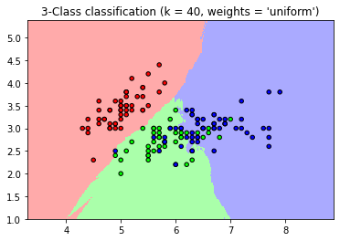

plot으로 그려진 결과 해석
- 거리(distance) 가중치의 KNN 분류의 의사결정 경계부분(Desicision Boundary)가 자연스럽움
- 직관적인 경계가 잘 나타나며 설명이 더 잘된 것으로 보임
- 하지만 이상치에 대한 분류를 제대로 하지 못함
** 결론적으로 가중치를 주는 결과가 항상 좋은 결과 값이 나오는 것이 아님
- 가중치의 유무에 따라 결과는 상충관계(Trade-off)가 있다
# 새로운 데이터셋을 생성
# SIN함수 예측

# 난수를 고정
np.random.seed(0)
X = np.sort(5 * np.random.rand(40, 1), axis=0)
T = np.linspace(0, 5, 500)[:, np.newaxis]
y = np.sin(X).ravel()
y[::5] += 1 * (0.5 - np.random.rand(8))

knn = neighbors.KNeighborsRegressor(n_neighbors)
y_ = knn.fit(X, y).predict(T)

# K = 5
n_neighbors = 5

for i, weights in enumerate(['uniform', 'distance']):
    knn = neighbors.KNeighborsRegressor(n_neighbors, weights=weights)
    y_ = knn.fit(X, y).predict(T)

    plt.subplot(2, 1, i + 1)
    plt.scatter(X, y, c='k', label='data')
    plt.plot(T, y_, c='g', label='prediction')
    plt.axis('tight')
    plt.legend()
    plt.title("KNeighborsRegressor (k = %i, weights = '%s')" % (n_neighbors,
                                                                weights))

plt.tight_layout()
plt.show()
- 가중치를 uniform에 둔 것이 가중치를 distance에 둔것 보다 더 sin 함수에 가까움
- 하지만 가중치를 distance에 둔것이 분포된 data를 세밀하게 따라감
'Python > 머신러닝' 카테고리의 다른 글
| 머신러닝 & AI 첫걸음 시작하기_마지막 (0) | 2022.06.14 |
|---|---|
| 머신러닝 & AI 첫걸음 시작하기_4 주차 (0) | 2022.06.07 |
| 머신러닝 인강을 무료로 듣기 위한 여정 (0) | 2022.05.14 |


